The Dry Martini Equation: Paul Desmond’s Alto Tone, Measured


A tone with a recipe
Paul Desmond once said he had wanted to “sound like a dry martini” (Quotewise), and nearly everyone who writes about him repeats the line. It survives because it is a specification. A dry martini is cold, clear, barely sweet and served without garnish. Desmond’s alto is the audio equivalent: a soft attack, pale upper partials, a narrow vibrato used sparingly, and dynamics that seldom push the reed into its loud, buzzy regime.
He was born Paul Emil Breitenfeld in San Francisco in 1924, co-founded the Dave Brubeck Quartet in 1951 and stayed until it disbanded in 1967 (Selmer). He wrote “Take Five,” the centerpiece of the 1959 album Time Out, which sold a million copies, and he died of lung cancer in 1977 at 52 (KCRW). Retrospectives describe the same contrast: a light, airy alto floating over Brubeck’s dense piano chords.
This piece treats the martini line as a hypothesis we can measure. A saxophone note is a physical signal with a harmonic spectrum, a pitch curve and an envelope, and “dry” maps onto a handful of numbers computed from those. I build the mapping from the acoustics up: the physics of a conical bore and a reed played softly, a feature extractor in Python, a classifier that learns which features separate a dry alto from a bright one, the neural models that can learn a timbre end to end, and the arithmetic of the 5/4 meter Desmond made famous. Every code block runs with numpy, scipy and scikit-learn, and every number in the text was recomputed from that code.
The frame: a note is a recipe of harmonics
A sustained saxophone note is, to a good approximation, a sum of harmonics: sine waves at whole-number multiples of the fundamental frequency f₀.
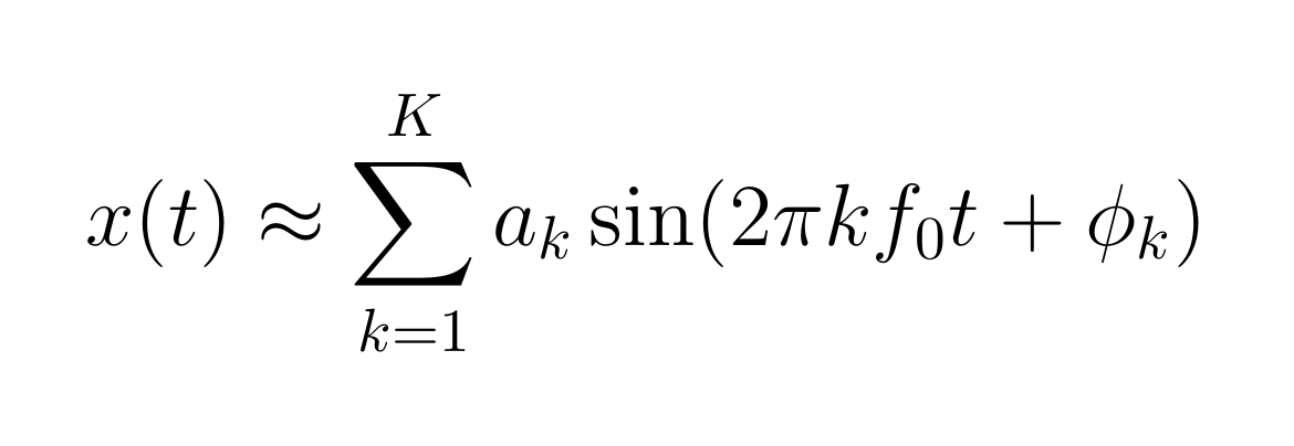
Here aₖ is the amplitude of harmonic k, φₖ its phase and K the number of harmonics that matter (18 below 8 kHz for a concert A4 at 440 Hz). On a steady tone the ear barely registers the phases. The amplitude recipe aₖ carries most of what we call the instrument’s color.
Psychoacoustics gives a principled way to collapse that recipe to one number. McAdams and colleagues had listeners rate how different 18 synthesized instrument tones sounded and found three perceptual dimensions: one tracked attack time, one tracked spectral variation over the note, and one tracked the spectral centroid, the amplitude-weighted mean frequency (McAdams et al., 1995).

To make “dry” concrete I use a proposed one-parameter model: harmonic amplitudes fall off as a power law, aₖ = k^(−β). A larger β means a steeper fall through the upper partials. Dividing through by f₀ leaves a centroid that depends only on β and K.

Plug in K = 18 and f₀ = 440 Hz. With β = 1, the spectrum of an ideal sawtooth wave, the centroid sits at 2,266 Hz, or 5.15 × f₀. With β = 2 it falls to 967 Hz, or 2.20 × f₀, a 57% drop. At β = 3 it is 583 Hz, barely above the fundamental. In this frame Desmond’s martini is a large β: most of the energy in the first three or four harmonics, the upper partials present but quiet.

At the 10th harmonic (4.4 kHz) the β = 1 tone is 20 dB below its fundamental and the β = 2 tone is 40 dB below. That 20 dB gap separates an edge you hear on every note from a shimmer you notice only when you listen for it.
One caveat on definitions. Some libraries weight the centroid by power (aₖ²) rather than amplitude, which is the same as doubling β and pulls every value toward f₀. Absolute numbers change between conventions, but the ranking of tones does not. Pick one convention and use it everywhere.
The physics: a cone, a reed and a quiet player
A saxophone has a full harmonic series to shape because its bore is a cone. With the tone holes closed, a conical pipe has input impedance peaks near f, 2f, 3f and upward, a complete harmonic series, where a clarinet’s cylinder favors the odd ones (UNSW Music Acoustics). The same page notes that above about 2.5 kHz the bore has no strong resonances left. My reading is that the top of the spectrum then depends mostly on how much harmonic energy the reed generates, which brings us to the player.
That is where Desmond’s dynamics come in. The reed is a pressure-controlled valve with a nonlinear flow curve. Played softly, it swings without slapping shut against the mouthpiece lay and the oscillation is close to sinusoidal. Played loudly, it beats against the lay, and the UNSW measurements show that blowing harder then barely changes the fundamental’s power while mainly adding high harmonics. Loudness and brightness are coupled in the instrument itself. A player who rarely leaves mezzo-piano gets a darker spectrum for free.
The classic way to quantify the soft regime is Worman’s rule, which Arthur Benade popularized: below the beating threshold, the amplitude of harmonic k grows roughly as the k-th power of the fundamental’s amplitude.

Here r is the factor by which the player scales the fundamental and ΔL is the change in level in dB. Halve the fundamental (r = 0.5, a 6 dB drop) and harmonic k falls a further (k − 1) × 6.02 dB relative to it: 6 dB more for the 2nd harmonic, 24 dB more for the 5th. Rolloff steepens as you play quieter, which is exactly a rising β. Worman’s rule predicts a roughly exponential fall with k rather than the power law in my frame, so treat β as a summary statistic, not a mechanism.
The mouthpiece adds a second, smaller lever. Desmond played a Selmer Paris Super Action alto (Selmer) with an M.C. Gregory Model A mouthpiece, a hand-finished piece with a thin beak, a medium chamber and usually a fairly closed tip (Saxophone.org). A medium chamber without a tall baffle adds little high-frequency emphasis, and a closed tip suits soft, controlled playing. None of that makes a Desmond sound by itself, but every piece of the setup points toward a high β.
The last component is the player’s own airway. Chen, Smith and Wolfe measured vocal tract impedance in saxophonists and found that professionals tune a strong tract resonance slightly above the note they play in the altissimo register, while amateurs do not (UNSW; Science 319, 2008). In the normal range the effect on timbre is real but much weaker for listeners than for the player. The useful lesson for modeling is that the source of a sax tone is the coupled system of reed, bore and airway, so a model trained only on the instrument’s output is learning a player, not a horn.
Measuring dry: a feature vector for one note
A single number will not hold the martini, so the extractor below returns a small vector per sustained note. It uses only numpy and scipy so it runs anywhere; librosa has equivalents for most of these if you already use it. Run it with no arguments to compare two synthetic tones, or pass a mono WAV of one held note.
Timbre features for a single sustained saxophone note.

Needs only numpy and scipy. Pass a mono WAV path, or run with no
arguments to compare two synthetic tones.
"""
import sys
import numpy as np
from scipy.io import wavfile
from scipy.signal import stft, butter, sosfiltfilt

def f0_track(x, sr, hop=256, win=2048, fmin=130.0, fmax=1000.0):
    """Frame-wise f0 by normalised autocorrelation (fine for a clean solo note)."""
    lags = np.arange(int(sr / fmax), int(sr / fmin))
    f0s = []
    for start in range(0, len(x) - win, hop):
        frame = x[start:start + win] * np.hanning(win)
        ac = np.correlate(frame, frame, mode="full")[win - 1:]
        ac /= ac[0] + 1e-12
        best = lags[np.argmax(ac[lags])]
        # parabolic interpolation around the peak for sub-sample accuracy
        y0, y1, y2 = ac[best - 1], ac[best], ac[best + 1]
        shift = 0.5 * (y0 - y2) / (y0 - 2 * y1 + y2 + 1e-12)
        f0s.append(sr / (best + shift))
    return np.array(f0s), sr / hop

def harmonic_amplitudes(x, sr, f0, n_harm=18):
    """Magnitude at each harmonic k*f0 from one long windowed FFT."""
    n = len(x)
    spec = np.abs(np.fft.rfft(x * np.hanning(n)))
    freqs = np.fft.rfftfreq(n, 1 / sr)
    amps = []
    for k in range(1, n_harm + 1):
        band = (freqs > k * f0 * 0.97) & (freqs < k * f0 * 1.03)
        # band energy, not the peak bin, so vibrato smearing does not bias high harmonics
        amps.append(np.sqrt((spec[band] ** 2).sum()) if band.any() else 0.0)
    return np.array(amps)

def features(x, sr, fmax=8000.0):
    x = x / (np.max(np.abs(x)) + 1e-12)
    f, _, Z = stft(x, sr, nperseg=2048, noverlap=1536)
    keep = f <= fmax                       # ignore the hiss-only band above fmax
    f, mag = f[keep], np.abs(Z[keep]) + 1e-12
    centroid = np.median((f[:, None] * mag).sum(0) / mag.sum(0))
    flatness = np.median(np.exp(np.log(mag).mean(0)) / mag.mean(0))
    cum = np.cumsum(mag, 0) / mag.sum(0)
    rolloff = np.median(f[np.argmax(cum >= 0.85, axis=0)])

    f0s, frame_rate = f0_track(x, sr)
    f0 = np.median(f0s)
    cents = 1200 * np.log2(f0s / f0)
    # vibrato: band-pass the pitch curve between 3 and 9 Hz
    sos = butter(2, [3, 9], btype="band", fs=frame_rate, output="sos")
    vib = sosfiltfilt(sos, cents)
    vib_extent = 2 * np.sqrt(2) * vib.std()          # peak-to-peak, cents
    spectrum = np.abs(np.fft.rfft(vib * np.hanning(len(vib))))
    vib_rate = np.fft.rfftfreq(len(vib), 1 / frame_rate)[np.argmax(spectrum)]

    a = harmonic_amplitudes(x, sr, f0)
    k = np.arange(1, len(a) + 1)
    # slope beta of a_k ~ k^-beta, fitted in log-log space
    beta = -np.polyfit(np.log(k), np.log(a + 1e-9), 1)[0]
    odd_even = a[0::2][1:].sum() / (a[1::2].sum() + 1e-12)   # 3,5,7.. over 2,4,6..
    return {
        "f0_hz": round(float(f0), 1),
        "centroid_hz": round(float(centroid), 1),
        "centroid_over_f0": round(float(centroid / f0), 2),
        "rolloff85_hz": round(float(rolloff), 1),
        "flatness": round(float(flatness), 4),
        "harmonic_slope_beta": round(float(beta), 2),
        "odd_even_ratio": round(float(odd_even), 2),
        "vibrato_extent_cents": round(float(vib_extent), 1),
        "vibrato_rate_hz": round(float(vib_rate), 1),
    }

def synth(beta, vib_cents, sr=44100, dur=2.0, f0=440.0, noise=0.01, seed=0):
    """Additive tone with a_k = k^-beta, sinusoidal vibrato and breath noise."""
    rng = np.random.default_rng(seed)
    t = np.arange(int(sr * dur)) / sr
    inst_f = f0 * 2 ** (vib_cents / 2 / 1200 * np.sin(2 * np.pi * 5.5 * t))
    phase = 2 * np.pi * np.cumsum(inst_f) / sr
    y = sum(k ** -beta * np.sin(k * phase) for k in range(1, 19))
    return y + noise * rng.standard_normal(len(t)), sr

if __name__ == "__main__":
    if len(sys.argv) > 1:
        sr, x = wavfile.read(sys.argv[1])
        x = x.astype(float)
        x = x.mean(1) if x.ndim > 1 else x
        print(features(x, sr))
    else:
        for name, beta, vib in [("bright, wide vibrato", 1.0, 40), ("dry, narrow vibrato", 2.0, 10)]:
            x, sr = synth(beta, vib)
            print(name, features(x, sr))
Two choices in that code matter more than they look. The harmonic amplitudes use the energy in a ±3% band around each k × f₀ rather than the single peak bin. Vibrato smears the upper harmonics across more bins than the lower ones, so a peak-bin measurement under-reads them; my first version, which used peaks, reported β = 1.42 for a tone built with β = 1. The second is the 8 kHz ceiling on the spectral features. Above it a real recording holds mostly hiss, and hiss drags the centroid upward.
On the two synthetic test tones (concert A4, 2 seconds, light added noise, 5.5 Hz vibrato) the extractor recovers the parameters it was given:

The measured centroids sit 6% and 12% above the analytic 2,266 Hz and 967 Hz. That gap is the noise floor, and it hits the dry tone twice as hard because a dry tone has less harmonic energy to outweigh the hiss. On real recordings, compare centroids only between notes with similar recording noise, or fit β, which is far less sensitive to it.
The time domain: vibrato and attack
Spectrum is only one of the three McAdams dimensions. The other two live in time, and they matter as much to the martini as β does. A dry tone is not only dark; it is also steady and soft-edged.
Start with vibrato. If the pitch oscillates as f(t) = f₀(1 + d sin 2πνt), the deviation in cents is what the ear compares across notes.

A 1% frequency swing (d = 0.01) is 17.2 cents either side of the center, 34 cents peak to peak. A 2% swing is 34.3 cents either side, about a third of a semitone. To my ear, Desmond’s sustained notes are mostly straight, with vibrato arriving late in a long note if at all. That is a hypothesis the extractor above can test, since it reports vibrato extent and rate for any held note. The interesting statistic is not one note’s extent but its distribution across a solo: how often the vibrato is near zero, and how late in the note it starts.
Attack is the other half. Log rise time was the first of the three McAdams dimensions, and a saxophonist controls it mostly through the tongue. A simple model of a soft onset is an exponential envelope e(t) = 1 − exp(−t/τ), whose 10% to 90% rise time is τ ln 9, about 2.2τ. A hard-tongued note might have τ = 5 ms (an 11 ms rise); a breathy legato onset might have τ = 20 ms (a 44 ms rise).
import numpy as np
from scipy.signal import hilbert

def rise_time(x, sr, lo=0.1, hi=0.9, smooth_ms=5.0):
    """10-90% rise time of the amplitude envelope, in milliseconds."""
    env = np.abs(hilbert(x))
    n = max(1, int(sr * smooth_ms / 1000))
    env = np.convolve(env, np.ones(n) / n, mode="same")
    peak = env.max()
    t_lo = np.argmax(env >= lo * peak)
    t_hi = np.argmax(env >= hi * peak)
    return 1000 * (t_hi - t_lo) / sr

if __name__ == "__main__":
    sr = 44100
    t = np.arange(int(0.5 * sr)) / sr
    for tau in (0.005, 0.020):
        x = (1 - np.exp(-t / tau)) * np.sin(2 * np.pi * 440 * t)
        print(f"tau = {tau*1000:.0f} ms -> rise {rise_time(x, sr):.1f} ms (theory {tau*1000*np.log(9):.1f})")
On the two test envelopes it reports 12.2 ms and 46.6 ms against theoretical values of 11.0 ms and 43.9 ms. The small overshoot comes from the 5 ms smoothing that keeps the Hilbert envelope from rippling at the carrier frequency; shrink it for fast attacks, at the cost of a noisier estimate. On a real solo, segment notes first (an onset detector or a transcription gives you the boundaries), then compute rise time per note and compare distributions between players rather than single values.
Spectral flux, the third dimension, ties the two domains together. A tongued attack on a reed instrument tends to be brighter for its first few tens of milliseconds than the steady state that follows. A player with soft attacks shows a smaller jump in centroid at onset. Computing centroid over the first 50 ms and over the sustain, and taking the ratio, gives a one-number proxy for how much of that bite a player allows.
Machine learning: from features to a learned timbre
Hand-built features answer “how dry is this note?” Machine learning answers two harder questions: which features actually separate Desmond from other altoists, and can a model learn his sound well enough to generate it.
The first obstacle is data. Desmond’s alto almost never appears alone on a record. Open-source separators help but do not solve it. Demucs v4 splits a mix into drums, bass, vocals and “other”; its six-source variant adds guitar and piano, but its own documentation calls the piano stem experimental, with heavy bleed and artifacts (Demucs on PyPI). In a Brubeck Quartet track the alto ends up in “other” with whatever piano the model failed to pull out. Separation artifacts also concentrate in the upper harmonics, which is exactly where β is measured. The defensible workflow is to separate, then keep only notes where the piano is silent or far below the alto, and to check β on a few hand-picked clean passages before trusting it at scale. Desmond’s own RCA quartet records with guitarist Jim Hall (KCRW), where the accompaniment is sparser, are a better starting corpus than Brubeck’s piano-heavy hits.
Once you have notes, a linear model is the honest first step, because its weights are readable. The script below trains logistic regression to tell a “dry” player from a “bright” one on the features from the previous sections. The data here is synthetic: two simulated players whose β and vibrato distributions overlap, across concert pitches from 220 to 700 Hz with varying noise. Swap synth() for real note clips and nothing else changes.
Which timbre features separate a 'dry' alto from a 'bright' one?

Synthetic stand-in data: swap synth() for notes cut from real recordings
(one sustained note per clip) and the rest of the pipeline is unchanged.
"""
import numpy as np
from sklearn.linear_model import LogisticRegression
from sklearn.model_selection import cross_val_score
from sklearn.pipeline import make_pipeline
from sklearn.preprocessing import StandardScaler

from dryness import features, synth

rng = np.random.default_rng(7)
FEATS = ["centroid_over_f0", "flatness", "harmonic_slope_beta", "vibrato_extent_cents"]

def player(n, beta_mu, vib_mu, label):
    rows = []
    for i in range(n):
        f0 = rng.uniform(220, 700)                  # concert pitches across the alto's range
        beta = rng.normal(beta_mu, 0.35)
        vib = max(0.0, rng.normal(vib_mu, 8))
        x, sr = synth(beta, vib, f0=f0, dur=1.0, noise=rng.uniform(0.005, 0.03), seed=i)
        feats = features(x, sr)
        rows.append([feats[k] for k in FEATS] + [label])
    return rows

data = np.array(player(80, 2.0, 12, 1) + player(80, 1.4, 28, 0))
X, y = data[:, :-1], data[:, -1]

clf = make_pipeline(StandardScaler(), LogisticRegression())
acc = cross_val_score(clf, X, y, cv=5)
print(f"5-fold accuracy: {acc.mean():.3f} +/- {acc.std():.3f}")

clf.fit(X, y)
for name, w in sorted(zip(FEATS, clf[-1].coef_[0]), key=lambda t: -abs(t[1])):
    print(f"{name:>22s}  {w:+.2f}")
It reaches 90.6% five-fold accuracy (±5.2 points). The standardized weights are the useful part: vibrato extent −3.71, harmonic slope β +1.58, centroid/f₀ −0.65, flatness +0.30. Vibrato does most of the work in this simulation, which is a property of the parameters I chose, not a finding about Desmond. The centroid’s small weight is the lesson worth keeping: centroid and β measure nearly the same thing, so a linear model splits the credit between them. Read weights on correlated features as a group, or drop one of the pair.
The end-to-end option is Differentiable Digital Signal Processing, from Engel, Hantrakul, Gu and Roberts at Google (DDSP, arXiv:2001.04643). Instead of generating raw samples, a small network drives a harmonic oscillator plus filtered noise, conditioned on f₀ and loudness. The oscillator’s amplitude is factored into an overall loudness and a normalized distribution over harmonics. That distribution is the aₖ recipe from the framing section, now predicted frame by frame by a neural net. The paper trained its violin model on about 13 minutes of one player.
Two things follow for a Desmond model. First, the data budget is reachable: a quarter hour of clean solo alto is plausible from separated, filtered tracks. Second, because the decoder maps loudness to a harmonic distribution, a trained model is an empirical Worman’s rule for one player. Sweep the loudness input with f₀ fixed, read off the predicted harmonics, fit β at each level, and you get a curve of how fast this player’s tone brightens as he plays louder. Comparing that curve between altoists is a sharper test of “dry” than any single spectrum.
A note on use. Analyzing a recorded timbre is research. Releasing synthetic performances in a named, deceased artist’s sound raises rights and consent questions that the code does not answer, so keep generated audio in the lab.
Rhythm and line: the arithmetic of five
The tone is only half of the Desmond signature that survives in the numbers. The other half is the piece everyone knows. Desmond composed “Take Five” after drummer Joe Morello pushed him to write in 5/4; it sits in E♭ minor over a two-chord vamp, and the five beats split 3 + 2, with the accents and chord changes on beats 1 and 4 (Wikipedia). It became the first jazz single to sell a million copies.
The choice of 3 + 2 was one of very few. To see how few, count the ways to split n beats into ordered groups of 2 and 3. Any such split ends in a 2 or a 3, which gives a recurrence.

This is a shifted Padovan sequence. Five beats allow exactly two groupings, 3 + 2 and 2 + 3. Seven allow three, nine allow five, and twelve allow twelve. The count grows by a factor approaching the plastic number, about 1.3247, the real root of x³ = x + 1. Odd meters are a small search space, which is part of why a few groupings recur across folk and popular music.
Godfried Toussaint showed that many traditional rhythms are Euclidean: k onsets spread as evenly as possible over n pulses (Toussaint, 2005). Two accents over five beats gives the pattern x . x . . (2 + 3), and “Take Five” uses its rotation x . . x . (3 + 2). Putting the long group first makes the bar lean forward into beat 4, which is one plausible reason the tune feels relaxed rather than lopsided.
On the melodic side, the cheapest useful statistic is the Shannon entropy of a solo’s interval distribution. A line built mostly from steps and a few favorite intervals has low entropy; a line full of varied leaps has high entropy.
"""Two small tools for the symbolic side: meter groupings and melodic entropy."""
from collections import Counter
from functools import lru_cache
import math

@lru_cache(maxsize=None)
def groupings(n):
    """Ways to split n beats into ordered groups of 2 and 3 (Padovan-style recurrence)."""
    if n < 0:
        return 0
    if n == 0:
        return 1
    return groupings(n - 2) + groupings(n - 3)

def interval_entropy(midi_pitches):
    """Shannon entropy, in bits, of the successive-interval distribution."""
    steps = [b - a for a, b in zip(midi_pitches, midi_pitches[1:])]
    counts = Counter(steps)
    total = sum(counts.values())
    return -sum(c / total * math.log2(c / total) for c in counts.values())

if __name__ == "__main__":
    for n in range(4, 13):
        print(n, groupings(n))
    # Toy lines, not transcriptions: a stepwise line and a leapy one over the same notes' range.
    stepwise = [63, 65, 66, 68, 66, 65, 63, 61, 63, 65, 66, 65, 63, 61, 60, 61]
    leapy = [63, 70, 61, 75, 66, 58, 68, 73, 60, 67, 75, 62, 70, 59, 66, 74]
    print(f"stepwise: {interval_entropy(stepwise):.2f} bits")
    print(f"leapy:    {interval_entropy(leapy):.2f} bits")
The two toy lines, 16 notes each and invented for the test, score 1.97 bits and 3.01 bits; 15 intervals that were all different would score log₂ 15 ≈ 3.91 bits. On real data the move is to compute this per solo for many players and see where a given altoist falls. The Weimar Jazz Database, an open collection of several hundred hand-transcribed jazz solos with audio, MIDI and Python tooling (MusoW entry), is the standard place to start. Check whether it holds the Desmond solos you want; if not, the extraction pipeline is the same on your own transcriptions. Entropy is a blunt tool. A next step is an n-gram or small transformer model of intervals trained per player, where per-note surprisal shows which moves are characteristic and which are rare.
Where it breaks
The biggest confound is the recording chain. Every Desmond note we can analyze passed through a 1950s to 1970s microphone, a console, tape, a mastering engineer and, usually, a later remaster. A modest high-shelf cut in a reissue can move the centroid as much as the gap between two players. The file holds Desmond multiplied by the room, the gear and the engineer. The defensible comparisons are within one recording, or between players captured in the same studio, era and label, and even those need a caution flag.
The power law is a summary, not the physics. Real saxophone spectra have bumps from bore resonances, and the UNSW measurements show a steeper envelope above a cutoff near 1.2 kHz on low notes. A fitted β compresses that shape into one number, and two quite different spectra can share a β. Fit β per register, and look at the residuals before trusting it.
Worman’s rule holds below the beating threshold and only roughly. Once the reed slaps the lay, the k-th power scaling breaks down, so the soft-playing derivation above explains the direction of Desmond’s sound, not its exact levels.
Perception is the gap no code closes. The McAdams dimensions came from synthesized tones rated in a lab, not from saxophone recordings, and “dry” is a metaphor. Whether listeners who call a tone dry are tracking β, vibrato, attack or something else is an empirical question that needs a listening test.
The classifier results in this piece come from simulated players. They show the pipeline works and how to read its weights; they say nothing yet about Desmond. Separation artifacts, which concentrate in the upper harmonics, can also bias β in either direction on real tracks.
Finally, the equipment details vary by source. The Selmer and Gregory facts above are well attested, but specific facings and chamber sizes reported online are inconsistent, and setup explains less of a sound than players usually hope.
The path forward
The martini line can be tested in a weekend. Pick 20 sustained notes from Desmond and 20 each from two altoists recorded in the same era and, ideally, the same studio. Cut each note to its steady portion, run the feature extractor, and compare the distributions of β, vibrato extent and rise time, not single values. If Desmond’s β sits clearly above his peers’ at matched pitch and loudness, the metaphor has a number.
The second experiment is the loudness curve. Group notes by measured level and fit β within each group. A player whose β falls slowly as he gets louder has a tone that stays dry under pressure, and that slope is likely more distinctive than any average. With a quarter hour of clean, separated alto from the Jim Hall quartet records, a DDSP model gives the same curve continuously.
The third is symbolic. Transcribe or source a set of solos, compute interval entropy and a per-player n-gram surprisal, and see whether the economy people hear in Desmond’s lines shows up as lower entropy than his contemporaries, or as something subtler, such as low entropy with rare, well-placed leaps.
For saxophonists the same tools work as a practice mirror. Record a long tone at three dynamics, run the extractor, and watch β and vibrato extent. Desmond got his sound with his ears, but a number that moves when your tone moves is a fast way to learn what your ears are hearing.
About the Author

Brian James Curry is a Kansas City AI researcher and data scientist, the founder of Vector1 Research, an independent applied AI lab, and the founder of KC AI Lab, which began in 2016 as the Kansas City Machine Learning Group and grew to more than 1,500 members. He has more than twenty years of experience leading analytics, data science and machine learning at enterprises including Hallmark, Garmin, Koch Industries, Tractor Supply Company and Vail Resorts. His open-source work, including Papilon, PyCausalSim, MeaningFlow, Daedalus and tincast, is on GitHub, and his research is published on Zenodo. He grew up in a small Kansas farming town and attended Kansas State University. He writes about causal inference, agent systems and the economics of AI on Medium and Substack. Contact: brian@vector1.ai.
Sources
- Paul Desmond, Henri Selmer Paris, artist page
- Paul Desmond: That Dry Martini Sound, KCRW, 2016
- Paul Desmond quote, Quotewise
- M.C. Gregory Model A, Saxophone.org mouthpiece museum
- Acoustics of the saxophone, UNSW Music Acoustics
- Saxophones and the vocal tract, J.M. Chen, J. Smith and J. Wolfe, UNSW (Science 319, 2008; JASA 129, 2011)
- Perceptual scaling of synthesized musical timbres, S. McAdams et al., Psychological Research 58, 1995
- DDSP: Differentiable Digital Signal Processing, J. Engel, L. Hantrakul, C. Gu and A. Roberts, arXiv 2001.04643, 2020
- Demucs, A. Défossez, PyPI documentation
- Take Five, Wikipedia
- The Euclidean algorithm generates traditional musical rhythms, G. Toussaint, Bridges, 2005
- Weimar Jazz Database, MusoW catalog entry


